Objective
One of the goals of image processing is Colour Reproduction. When placed in a real scene, the light received can originate from reflection, transmission, scattering, or a mixture of these from different objects, or directly from light sources. Their spectra vary greatly, and their luminance can span a wide range. Displays, on the other hand, can only provide a limited luminance range and spectroscopically can only offer a mixture of three primaries.
Fortunately, metamerism and the complexity of visual colour perception make Colour Reproduction possible. Through the research and development in colour science, what we pursue is no longer merely the reproduction of luminance or colour coordinates, but the reproduction of Colour Appearance. This requires the involvement of Colour Appearance Models.
Colour Appearance Models can be used to predict the Colour Appearance (Lightness, Chroma, etc.) of a tristimulus value under specific Viewing Conditions. For image and Colour Reproduction, it is necessary to consider the vastly different Viewing Conditions between the real scene and the Display. Traditional cinemas can only provide a luminance of about 48 nits, yet they can reproduce vivid scenes. This is partly because cinemas provide a nearly dark, low-luminance Viewing Condition.
By using a forward Colour Appearance Model, the Colour Appearance of each pixel is calculated from its tristimulus values. Then, based on the Viewing Conditions of the Display, an inverse Colour Appearance Model is applied to predict what tristimulus values the Display needs to produce to achieve that Colour Appearance. This constitutes a relatively complete image processing pipeline for Colour Reproduction using Colour Appearance Models.
iCAM06 is a Colour Appearance Model proposed by Jiangtao Kuang et al. for rendering HDR images. It incorporates many theories and algorithms from Colour Appearance Models, achieving a relatively scientific image processing approach from scenes with a large luminance range to Displays.
Starting Point: Input
A typical Colour Appearance Model accepts tristimulus values and Viewing Conditions as input.
Tristimulus values differ from the more common RGB space; they are a device-independent space. They are independent of the device, and under the same Viewing Conditions, if two colours have equal tristimulus values, they will achieve a match (look the same). RGB is a device-dependent space; for example, if two different Displays both display a pure red, the RGB values might be equal, but the colours are likely different because different Displays have different red primaries.
In a traditional image processing workflow, starting from a raw image and going through White Balance and Colour Correction Matrix (CCM), the colour space can be converted to XYZ tristimulus values. A common implementation is in the raw image processing library rawpy, where output_color = rawpy.ColorSpace(5) specifies the output colour space.
It is important to note that the XYZ values obtained this way are not the tristimulus values of the actual scene but are already White Balanced (Chromatic Adapted) tristimulus values. What we need are colours that represent the actual scene; therefore, a slightly modified initial ISP is required.
From a more fundamental perspective, how is a raw image generated from the spectrum?
$$ R=\int P(\lambda)\,\bar{r}(\lambda)\,\mathrm{d}\lambda $$The equation above represents an ideal image Sensor’s expression, where $P$ is the spectral power, $\bar{r}$ is the Sensor’s Spectral Sensitivity Function, determined by the spectral characteristics of the photodiode, the transmittance of the colour filter, etc. $R$ is the output pixel value, which can be read from the raw file.
The expression for tristimulus values can be written as:
$$ X=\int P(\lambda)\,\bar{x}(\lambda)\, \mathrm{d}\lambda $$Here, $\bar{x}$ represents the Spectral Sensitivity Function of the human eye. Therefore, if we can linearly combine $\bar{r}(\lambda),\bar{g}(\lambda),\bar{b}(\lambda)$ to produce $\bar{x}(\lambda)$, etc., we can estimate the tristimulus values using the camera’s raw pixel values. This linear combination process can be represented by a 3x3 matrix.

The image above illustrates using a linear combination to predict tristimulus values from the camera’s Spectral Sensitivity Functions. The camera’s Spectral Sensitivity Functions after linear combination have shapes similar to the Colour Matching Functions of the tristimulus values.
Additionally, a coefficient is needed for scaling to convert to tristimulus values representing Absolute Luminance. This coefficient can be calculated from the camera’s Aperture, Shutter Speed, and ISO. These parameters used to control the amount of light entering do not affect the linearity or relative relationships of the light.
Another scenario involves using High Dynamic Range Images as input, such as HDR images encoded with the PQ Transfer Function. First, the non-linearly encoded RGB pixel values are decoded using the EOTF to obtain linear RGB pixel values. Then, the linear RGB pixel values are converted to the XYZ space to obtain the tristimulus values. Several of the .tif files and image_input.py provided in the project utilize this type of input.
Image Decomposition
According to the visual system’s different perception of colour and detail, the image is decomposed into a Base Layer and a Details Layer. Operations on colour, such as Chromatic Adaptation and Tone Compression, are only applied to the Base Layer. The Details Layer, after enhancement or adjustment, is merged with the adjusted Base Layer.
The Base Layer is obtained using an edge-preserving Bilateral Filter, a method previously proposed by Durand and Dorsey. Bilateral Filtering is a non-linear filter where the weight of each pixel is jointly determined by a Gaussian filter in the spatial domain and another Gaussian filter in the intensity domain. The latter reduces the weight of pixels with significant intensity differences from the center pixel.
Therefore, Bilateral Filtering can effectively smooth the image while preserving sharp edges, thereby avoiding the “halo” artifacts common in local tone mapping operators. The intensity domain calculations are performed in Logarithmic Space, where intensity better represents perceived contrast and facilitates more uniform processing across the entire image.
The Details Layer is obtained by subtracting the Base Layer from the original image. Both layers need to be converted back to linear space.
The Bilateral Filtering used in iCAM06 is accelerated through piecewise linear approximation and nearest-neighbor downsampling.

Chromatic Adaptation
The colour of an object changes under different lighting and Viewing Conditions, but the human visual system can maintain a relatively stable perception of the object’s colour to some extent. This phenomenon is called Colour Constancy. This process of maintaining relative stability is called Chromatic Adaptation.
A Chromatic Adaptation Transform (CAT) is a model used to predict corresponding colours. It takes two Viewing Conditions (usually represented by the tristimulus values of the scene white point) and a colour under one Viewing Condition as input, and predicts the colour under the other Viewing Condition that would be a corresponding colour.
According to von Kries’ hypothesis, Chromatic Adaptation is independent at the level of the visual organs. The basic structure of a Chromatic Adaptation Transform is:
- Convert the input XYZ to a space representing the visual organs (Cone responses).
- Process each quantity independently in this space (e.g., multiply by respective gain factors).
- Convert back to XYZ space to obtain the colour tristimulus values under the other Viewing Condition.
There are many Chromatic Adaptation Transforms designed according to this structure, among which CAT02 and CAT16 are two CAT models successively recommended by CIE. In the second step, there is an adaptation degree D, representing the extent of Chromatic Adaptation. In iCAM06, this adaptation degree is multiplied by a coefficient of 0.3, which is equivalent to reducing the degree of adaptation, bringing it closer to the colours in the scene rather than the adapted corresponding colours, to increase the colour saturation of the image.
This is a very strange practice. I am more inclined to believe it is a code error that causes numerical errors if this coefficient is not multiplied. This is because the two Cone responses used in the Chromatic Adaptation step in the original code are one normalized and one absolute value.
In iCAM06, the target adaptation field for this step of Chromatic Adaptation is D65, because the subsequent uniform colour spaces are designed for the D65 white point. The white point of the adaptation field uses a Gaussian blur of the Base Layer, which is somewhat similar to the Grey World hypothesis.
$$ \begin{align*} D &= 0.3 F \left[ 1 - \left( \frac{1}{3.6} \right) e^{-\frac{(L_A - 42)}{92}} \right] \\ R_c &= \left[ \left( R_{D65} \frac{D}{R_W} \right) + (1-D) \right] R \end{align*} $$In the original equation, the sign of 42 in the exponent of $e$ in the calculation of adaptation degree D is incorrect.
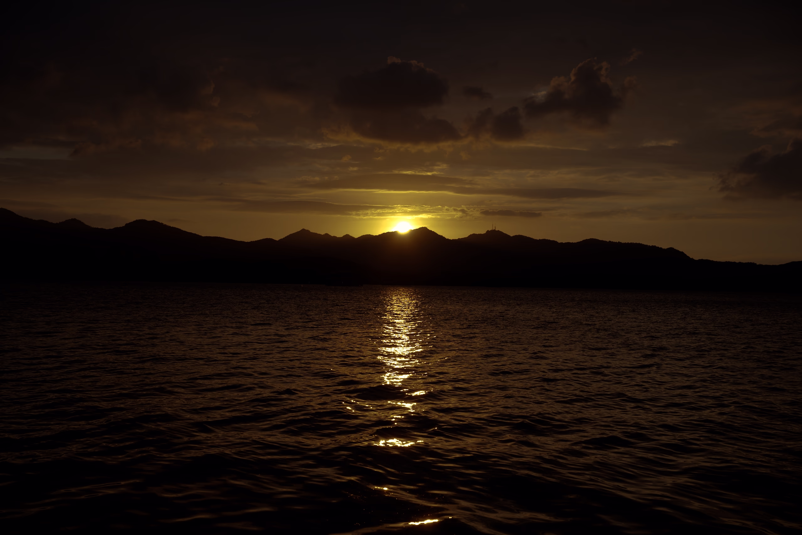
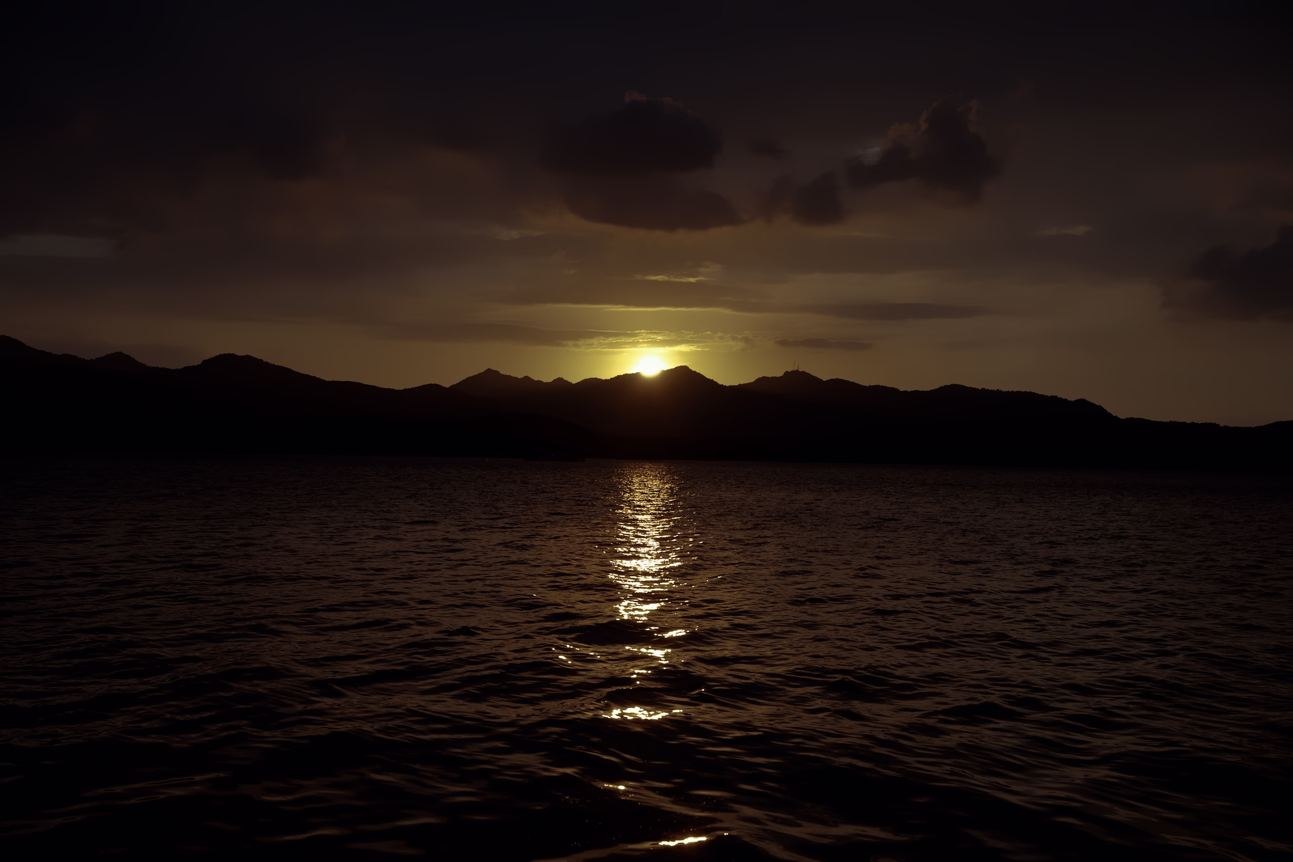
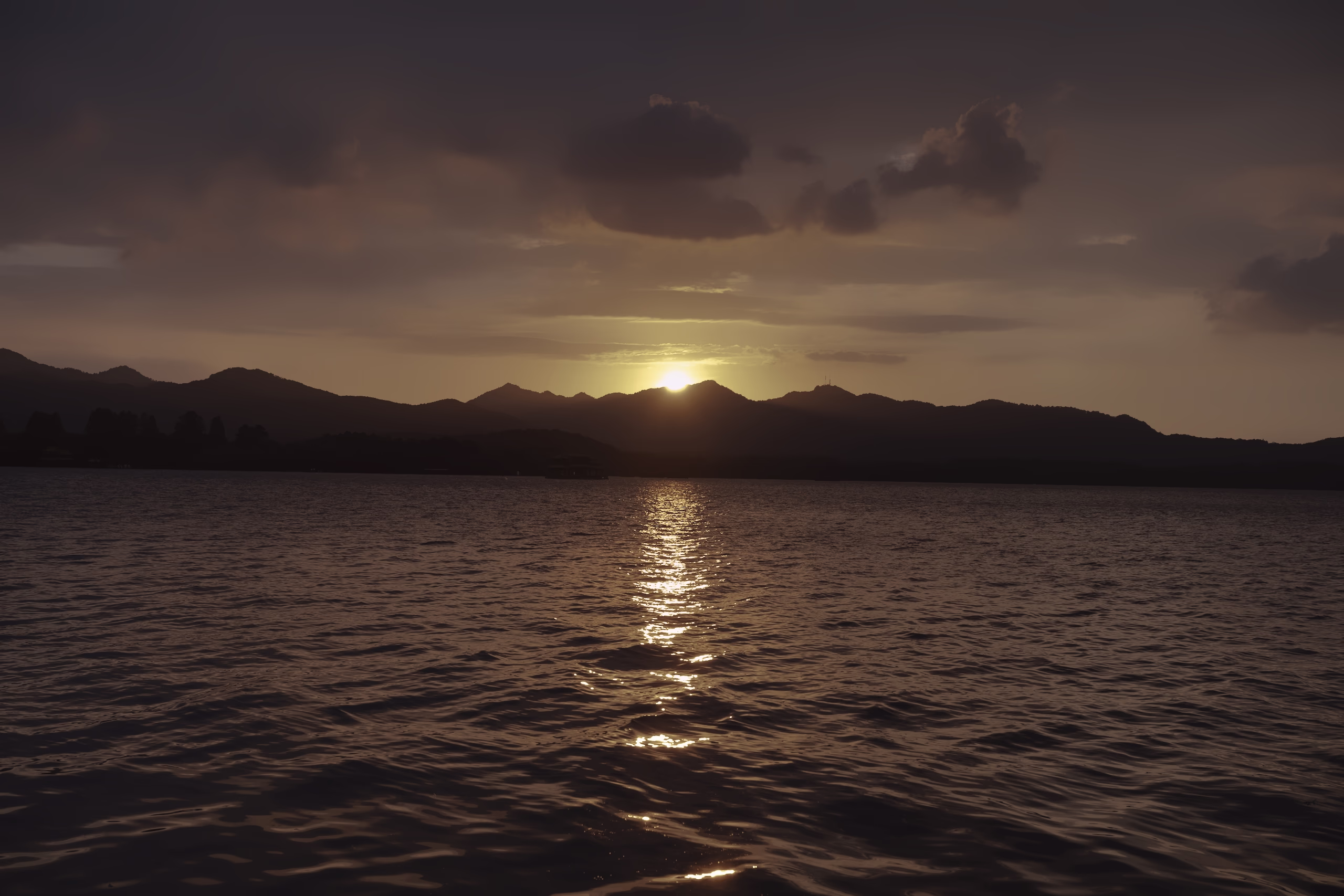
 The Adaptation White (Above) and Adapted Image (Below)
Tone Compression
The human eye’s perception of luminance is not linear, but highly non-linear. By applying Tone Compression according to this non-linear characteristic, it is possible to reproduce Colour Appearance with a larger luminance range within a limited Display luminance range.
This non-linear relationship is also obtained from visual experiments. iCAM06 uses the post-adaptation part from CIECAM02, which is shaped like a Sigmoid function. When used, it involves converting from tristimulus values to another space representing visual cells, and then applying a response curve called “post-adaptation”. In iCAM06, the response of Rods under scotopic vision is also added and superimposed on the Cone response to predict luminance in the scotopic-mesopic range; the Rod response is very small.
The post-adaptation non-linear relationship for Cones is as follows:
$$ R'_a = \frac{400 (F_L R' / Y_W)^p}{27.13 + (F_L R' / Y_W)^p} + 0.1 $$The reference white $Y_{W}$ used in this step is also a Gaussian blur of the Base Layer, but with a greater degree of blur than in Chromatic Adaptation.
This step completes the compression of luminance. The original large luminance range, after passing through this Sigmoid function, has a range of 0.1 to 400, although it rarely exceeds 200. Before this step, the relationship was linear with the scene light; after this step, it is linear with the Display light. Therefore, this step can also be understood as an Optic-Opto Transfer Function (OOTF).
Merging Image and Output
After completing Chromatic Adaptation and Tone Compression, the Base Layer is an image that can be displayed relatively normally on a screen. The Details Layer can be enhanced and merged back.
The image obtained at this point is still in the linear XYZ tristimulus value space. Converting XYZ to the RGB space suitable for display involves two steps:
- Conversion to linear RGB space.
- Applying the Transfer Function encoding.
For the most common sRGB space, the matrix used in the first step is readily available online. The second step is a Gamma Correction, with a coefficient equal to the reciprocal of the Display’s Gamma, usually between 0.45 and 0.5.
Additional Operations: IPT Space
Compressing an original high dynamic range, high luminance image onto a low luminance Display can sometimes result in less vivid colours, and the contrast between light and dark areas also needs to be enhanced.
The solution in iCAM06 is to convert to a uniform colour space for enhancement, choosing the IPT space. I represents Lightness, and P and T represent two colour directions, red-green and yellow-blue respectively.
The method for enhancing contrast is to apply a Gamma exponent between 1.0 and 1.5 to Lightness, with the value determined by the Viewing Environment. The principle is that perceived contrast changes according to the relative luminance of the Viewing Environment. Dark environments like cinemas require higher contrast, so a higher System Gamma exponent is usually adopted. A potential issue is that past System Gamma was applied to linear light, not to a non-linear scale like Lightness.
The method for enhancing Chroma is to stretch the two colour directions. The degree of stretching is related to luminance, based on the Hunt effect: an increase in luminance leads to an increase in perceived Colourfulness.
$$ P = P \cdot \left[ (F_L + 1)^{0.2} \left( \frac{1.29C^2 - 0.27C + 0.42}{C^2 - 0.31C + 0.42} \right) \right] $$
Results and Analysis
This algorithm addresses two problems:
- How to reproduce real-world scenes on a display.
- How to reproduce high dynamic range images on traditional low dynamic range displays.
Unlike computer vision, colour science focuses more on human visual perception, aiming to process images from a visual perspective. iCAM06, through methods such as Chromatic Adaptation, Tone Compression, and uniform colour spaces, provides an interpretable solution for image processing from high dynamic range to low dynamic range.
However, iCAM06 also has some shortcomings:
- The Chromatic Adaptation algorithm has issues, and the effect after correction is not ideal, possibly due to the limitations of the Chromatic Adaptation model and the influence of the Grey World hypothesis.
- The Sigmoid function used for Tone Compression reduces image contrast too much and cannot balance the effects for both low dynamic range and high dynamic range inputs.
- Edge-preserving transformation and detail enhancement may introduce artifacts and excessive sharpening.
- Processing in a uniform colour space lacks reliable theoretical basis, especially the practice of applying a gamma exponent to Lightness.
Overall, iCAM06, leveraging research from colour science, proposes an effective method for high dynamic range image processing and is a successful exploration of integrating colour science into image processing.
References
[1] M. D. Fairchild and G. M. Johnson, “Meet iCAM: A next-generation color appearance model,” Proc. 10th Color Imaging Conf., vol. 10, no. 1, pp. 33–38, Jan. 2002.
[2] J. Kuang, G. M. Johnson, and M. D. Fairchild, “iCAM06: A refined image appearance model for HDR image rendering,” J. Visual Communication and Image Representation, vol. 18, no. 5, pp. 406–414, Oct. 2007.
[3] F. Durand and J. Dorsey, “Fast bilateral filtering for the display of high-dynamic-range images,” in Proc. 29th Annual Conf. Computer Graphics and Interactive Techniques (SIGGRAPH), San Antonio, TX, USA, Jul. 2002, pp. 257–266.
[4] P. Hung and R. S. Berns, “Determination of constant hue loci for a CRT gamut and their predictions using color appearance spaces,” Color Research & Application, vol. 20, no. 5, pp. 285–295, Oct. 1995.
[5] M. R. Luo and C. Li, “CIECAM02 and its recent developments,” in Advanced Color Image Processing and Analysis, C. Fernandez-Maloigne, Ed., New York, NY, USA: Springer, 2013, pp. 19–58.
[6] M. D. Fairchild, “A revision of CIECAM97s for practical applications,” Color Research & Application, vol. 26, no. 6, pp. 418–427, 2001.