For more information on chromatic adaptation and chromatic adaptation models, please refer to section 1.2.1 of this paper:
Q. Zhai, ‘Chromatic Adaptation to Illumination and Colour Quality’, PhD dissertation, Zhejiang University, 2018.
Colour Constancy
The colour of an object changes under different lighting conditions and viewing environments, but the human visual system can maintain a stable perception of the object’s colour to a certain extent. This phenomenon is known as colour constancy. The process of maintaining this relative stability is called chromatic adaptation.
When the lighting environment changes, chromatic adaptation takes some time to complete. The figure shows the experimental results from Fairchild and Reniff (1995), illustrating the relationship between the proportion of steady-state adaptation and time for three observers, switching from illuminant A to D65.
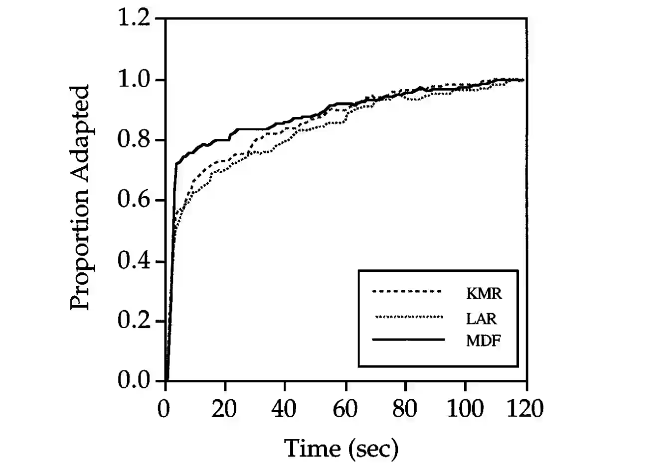
M. D. Fairchild and L. Reniff, ‘Time course of chromatic adaptation for color-appearance judgments’, J. Opt. Soc. Am. A, vol. 12, no. 5, p. 824, May 1995, doi: 10.1364/JOSAA.12.000824.
The formation mechanism of chromatic adaptation can be broadly divided into two parts: sensory and cognitive.
The sensory mechanism suggests that the three types of cone cells on the retina automatically and independently adjust their gain according to the intensity of light. When the response of a certain type of cone cell increases, its gain is reduced, and the gain adjustments of the three types of cone cells are independent. The fundamental hypothesis proposed by von Kries in 1902 posits that the fatigue or adaptation of each component of the visual organ is independent of the others (the concept of cone cells did not exist at the time). The von Kries hypothesis is the foundation of all chromatic adaptation models.
“This can be conceived in the sense that the individual components present in the organ of vision are completely independent of one another and each is fatigued or adapted exclusively according to its own function.”
The cognitive mechanism is more complex and suggests that a person’s perception of an object’s colour is also influenced by the object itself. For example, grass is green, apples are red, and the sky is blue; vision can maintain a stable perception of the colours of these objects under various lighting conditions. The formation of this cognitive mechanism may be due to the accumulation of experience with object colours over a lifetime. Chromatic adaptation resulting from cognitive mechanisms is often incomplete.
A typical example of a cognitive mechanism is ‘discounting the illuminant’. This refers to the ability of an observer to judge an object’s colour based on its inherent properties (reflectance) rather than the light source. For instance, coal is black during the day and snow is white at night, but in reality, the luminance of coal during the day is higher. The visual system perceives primarily the reflectance of the coal and snow. Discounting the illuminant is very important in cross-media colour reproduction. Cross-media colour reproduction refers to displaying colours using different media, such as a self-luminous display and colours printed on paper. The self-luminous display is itself a light source, so there is no phenomenon of discounting the illuminant, whereas for printed colours, the observer can, to some extent, ignore the influence of the illuminating light source.
Apple’s True Tone technology, introduced on the iPhone 8 and iPhone X, adjusts the display’s colour based on changes in ambient lighting. This simulates the phenomenon of discounting the illuminant, making the display appear like a printed paper under the same light source, which enhances viewing comfort to some extent.
Chromatic Adaptation Transform
A chromatic adaptation transform establishes a relationship between ‘corresponding colours’. Corresponding colours are two colours that match under different viewing conditions. Imagine an observer with perfect colour constancy; if the light source in a scene is changed, the colour they perceive remains the same (i.e., it always matches). In this case, the colours of the same object under the different light sources form a pair of corresponding colours. Colours are typically represented by their XYZ tristimulus values. If the tristimulus values under the first viewing condition are $X_1, Y_1, Z_1$, and under the second viewing condition are $X_2, Y_2, Z_2$, then these two sets of tristimulus values are corresponding colours for those two viewing conditions.
A Chromatic Adaptation Transform (CAT) is a model used to predict corresponding colours. The inputs are two viewing conditions (usually represented by the tristimulus values of the scene white point), and a colour under one of the viewing conditions (represented by its tristimulus values). The model predicts the colour under the other viewing condition that forms a corresponding pair (also represented by tristimulus values).
Building a CAT model requires corresponding colour datasets for training and validation. The following are some common experimental methods for creating these datasets:
- Haploscopic matching: An experimental apparatus is designed to separate the visual fields of the left and right eyes, placing them under different viewing conditions. The observer then compares and matches the colour stimuli from both sides. This method cannot be used to study chromatic adaptation caused by cognitive mechanisms.
- Memory matching: The subject memorises a colour stimulus under one viewing condition and then matches it under another viewing condition.
- Magnitude estimation: The subject ‘rates’ colour stimuli in different viewing environments, for example, by estimating numerical values for lightness, saturation, hue, etc.
I have not designed, conducted, or participated in any experiments on chromatic adaptation. From a purely subjective perspective, I believe collecting corresponding colour data is very difficult. Each of the three methods mentioned above has its own drawbacks. For instance, in memory matching, human short-term memory for colour is very limited. In magnitude estimation, having subjects assign scores to a subjective value requires careful experimental design to standardise the rating criteria among subjects.
Basic Structure of a CAT
According to the von Kries hypothesis, chromatic adaptation is independent at the level of the visual organs. The basic structure of a chromatic adaptation transform is as follows:
- Transform the input XYZ values into a space that represents the visual organs.
- Process each component independently within this space (e.g., by multiplying by its respective gain coefficient).
- Transform back to the XYZ space to obtain the colour tristimulus values for the other viewing condition.
Von Kries himself never provided a specific CAT method, but simple chromatic adaptation models, such as the Ives and Helson models, can be built based on his hypothesis.
M. H. Brill, ‘The relation between the color of the illuminant and the color of the illuminated object’, Color Research & Application, vol. 20, no. 1, pp. 70–76, Feb. 1995, doi: 10.1002/col.5080200112.
H. Helson, ‘Some Factors and Implications of Color Constancy*’, J. Opt. Soc. Am., vol. 33, no. 10, p. 555, Oct. 1943, doi: 10.1364/JOSA.33.000555.
First, the light sources or white points of the two viewing conditions and one colour stimulus (\(\text{XYZ}_{w1}, \text{XYZ}_{w2}, \text{XYZ}_{1}\)) are transformed into the LMS relative cone response space. This can be done using a 3x3 matrix. Then, each component is multiplied by a gain coefficient, which can be represented as multiplication by a diagonal matrix. Finally, the values are transformed back to the XYZ space by multiplying by the inverse of the first matrix, yielding $\text{XYZ}_{2}$, sometimes written as $\text{XYZ}_c$ to denote the corresponding colour.
The gain coefficients are the ratio of the cone responses to the light sources or white points of the two viewing conditions, reflecting the hypothesis that ‘a visual organ with a larger stimulus will automatically adjust to reduce its gain’. For example:
$$ L_2 = \frac{L_{w2}}{L_{w1}} L_1 $$Such simple linear models are already capable of predicting the data in corresponding colour datasets quite well.
Improvements to CATs
Some research has proposed using non-linear adjustments or non-independent adjustments with cross-channel interactions in the second step to try to improve chromatic adaptation transforms. For example, Nayatani and Guth used a power function instead of linear gain. However, these methods did not achieve significantly better results.
Changing the transformation matrix from XYZ tristimulus values to the LMS relative cone space may yield better results. In this case, the space is no longer referred to as LMS, but as RGB. Examples include the HPE transformation matrix used by Fairchild, the BFD transformation matrix by Bradford, and the matrices used in CAT02 and CAT16.
Additionally, although non-linear adjustments do not yield better results, improvements can be made to the coefficients used in linear gain. For example, CMC-CAT and CAT02 introduced the concept of a degree of adaptation, D, to control the completeness of the adaptation. D ranges between 0 and 1, where 1 represents complete adaptation and 0 represents no adaptation. In CAT02, D is a value related to the luminance of the adapting field on the input side, and a factor F, representing the ambient surround (bright or dark), is also included.
$$ D = F \cdot \left[1 - \frac{1}{3.6} e^{\frac{-L_A - 42}{92}}\right] $$Here, $L_A$ is the luminance of the adapting field on the input side in cd/m², and $F$ is the surround factor. It is set to 1.0 for an average surround, 0.9 for a dim surround, and 0.8 for a dark surround. The choice is determined by the relative luminance, for example, a bright office, watching television indoors, or a dark cinema.
CAT16
The current CIE recommended chromatic adaptation transform is CAT16, which is a linear transform. The process for the one-step CAT16 is as follows.
Inputs: White point of the input adapting field \(\text{XYZ}_{w}\), white point of the output (reference) adapting field $\text{XYZ}_{wr}$, input colour $\text{XYZ}$, luminance of the adapting field light source $L_A$, and surround factor $F$.
-
Transform \(\text{XYZ}_{w}\), \(\text{XYZ}_{wr}\), and $\text{XYZ}$ into the RGB space using the transformation matrix \(\mathbf{M}_{16}\).
\[ \begin{bmatrix} R \\ G \\ B \end{bmatrix} = \begin{bmatrix} 0.401288 & 0.650173 & -0.051461 \\ -0.250268 & 1.204414 & 0.045854 \\ -0.002079 & 0.048952 & 0.953127 \end{bmatrix} \begin{bmatrix} X \\ Y \\ Z \end{bmatrix} \] -
Perform the adaptation transform on each of the three RGB channels separately. The gain coefficients depend on the degree of adaptation, D, which is calculated in the same way as in CAT02. For the G and B gain coefficients, $R_{wr}$ and $R_w$ are replaced accordingly.
\[ k_R = D \cdot \frac{Y_w}{Y_{wr}} \cdot \frac{R_{wr}}{R_w} + 1 - D \\ R_c = k_R \cdot R \] -
Transform the adapted RGB values back to the XYZ space using \(\mathbf{M}_{16}^{-1}\). The subscript c or r is used to denote the corresponding colour or the reference field, respectively.
\[ \begin{bmatrix} X_c \\ Y_c \\ Z_c \end{bmatrix} = \mathbf{M}_{16}^{-1} \begin{bmatrix} R_c \\ G_c \\ B_c \end{bmatrix} \]
Due to the presence of the degree of adaptation D, CAT16 is not reversible in most cases. There is also a two-step version of CAT16 designed to solve the problem where the original input cannot be recovered after inverting the one-step method. The two-step method defines an intermediate illuminant, such as an equal-energy white, and works by adapting the input field to the equal-energy white field and then predicting the corresponding colour for the output field in reverse from the equal-energy white field.
If we use \(\Lambda_{r,t}\) to denote the linear gain diagonal matrix from the input field t to the output field r, then the total transformation matrix for the one-step method is:
\[ \Phi_{r,t} = \mathbf{M}_{16}^{-1} \Lambda_{r,t} \mathbf{M}_{16} \]The total transformation matrix for the two-step method is:
\[ \begin{align*} \Pi_{r,t} &= \Psi_{r,se} \Phi_{se,t} \\ &= \mathbf{M}_{16}^{-1} \Lambda_{se,r}^{-1} \mathbf{M}_{16} \mathbf{M}_{16}^{-1} \Lambda_{se,t} \mathbf{M}_{16} \\ &= \mathbf{M}_{16}^{-1} \Lambda_{se,r}^{-1} \Lambda_{se,t} \mathbf{M}_{16} \end{align*} \]Here, ‘se’ denotes the equal-energy white. In practice, there is almost no difference in the results between the two-step and one-step methods, and the one-step method is currently more commonly used.